LPRM: a user-friendly iteration-free combined Local Polynomial and Rational Method toolbox for measurements of multiple input systems
Goals
Scientists and engineers want accurate mathematical models of physical systems for understanding, design, and control. This work presents a user-friendly signal generation Matlab toolbox for real-life (industrial) experiments of physical systems. This work. introduces a user-friendly estimation toolbox for (industrial) measurements of (vibro-acoustic) systems with multiple inputs. The vibration testing methods are very important because they help to improve the product quality and to avoid safety and comfort issues. The time-consuming testing procedures are nowadays fully substituted by techniques that evaluates the frequency response functions (FRFs). The toolbox provides a user-friendly nonparametric estimation method that uses a special combined Local Polynomial/Rational approach. The toolbox can be used even in case of multiple inputs with only one measured period – that would be not possible with the classical FRF estimator frameworks.Introduction
This paper presents a user-friendly nonparametric transfer function estimation toolbox for (industrial vibro-acoustic) measurements with multiple inputs. The vibration testing methods are very important because they help to improve the product quality and to avoid safety and comfort issues. The increasing needs for higher accuracy and faster testing techniques inspirited a lot of international researchers. Since the development of advanced digital signal processing algorithms and the increased computational capability, it became possible to use complex methods to determine the broadband frequency response functions (FRFs). As a result, time-consuming testing procedures are nowadays almost fully substituted by techniques that evaluates the FRFs. In this work the considered systems are dynamic vibro-acoustic systems such as mechanical, civil structures, passive electronics (and thermodynamic systems with resonances in the frequency domain). The dynamics of a linear multiple input, multiple output (MIMO) system can be nonparametrically characterized in the frequency domain by its Frequency Response Matrix (FRM, a matrix whose elements are FRFs) G at frequency index k, which relates the inputs U to the outputs Y of N measurement samples as follows:Y[k]=G[k]U[k]
where k=0…(N-1)/2 at frequency fk=kfs/N, sampling frequency of fs.
In this framework it is assumed that the output Y is measured with additive, independent and identically distributed Gaussian noise with zero mean and finite variance (denoted as E), and it (can) contain transient response (denoted as T) such that the measurement Ymeas is given by:
Ymeas [k]=Y[k]+E[k]+T[k]=G[k]U[k]+E[k]+T[k]
For most of the nonparametric FRF estimation methods it is crucial that the steady-state signals are considered, otherwise the transient term is included in the estimated FRF model that results in higher bias (and variance) error and therefore it will be not an adequate representation of the system. The transient term occurs when the system is initially not at rest, when the past values of the excitation signal are unknown, when there is a change in the excitation signal or when fade-in/fade-out is used. When multiple inputs are present, the necessary measurement time can be extremely long. To overcome these issues, the author proposes an iteration free, (simple) combined Local Polynomial and Rational method.
When many periods of data are available, it is the best practice to discard the first few blocks (the transient periods or in other words, the delay blocks). When it is not possible, different windowing methods are used in practice [1] [8] [9]. The methods still suffer from higher bias (and variance) errors.
To overcome these issues, more advanced techniques have to be used. Because the FRF and the transient are smooth it is possible to use polynomial approximations. In this work special (straightforward, iteration free, direct) combined implementation of Local Polynomial and Local Rational Method (LPM and LRM) are considered.
The drawback of the LPM is that it has issues with highly damped systems such that the peaks in the FRFs are usually underestimated. To improve the estimates at a cost of more parameters to be estimated LRM method can be used. The LRM still uses the property of the smoothness of the FRF and transient but also uses the fact that they inherently have common poles (which is the difference between LPM and LRM). The drawback is that LRM requires a good signal-to-noise ratio (SNR) of the output measured signal. In the estimation process, a sliding processing window is used with a polynomial degree of d. First, an excited frequency line is selected (frequency index k), this is called the central frequency, this is the middle point of the processing window. Around this frequency line in a r=±d/2 radius a narrow band is selected. In this band the FRFs are estimated in polynomial form. An illustration of the method is shown in the figure below. The measured output is given by at the excited frequency index k in a radius of r as follows:
Ymeas[p][k+r]=G[p][k+r] U[p] [k+r]+T[k+r][p][k+r]+E[p][k+r]=GpU[p])/D+Tp/D+E[p][k+r]
where Gp, Tp, D are polynomials of order d, k is an excited frequency line (here it is the so-called central frequency), and r is a narrow band.
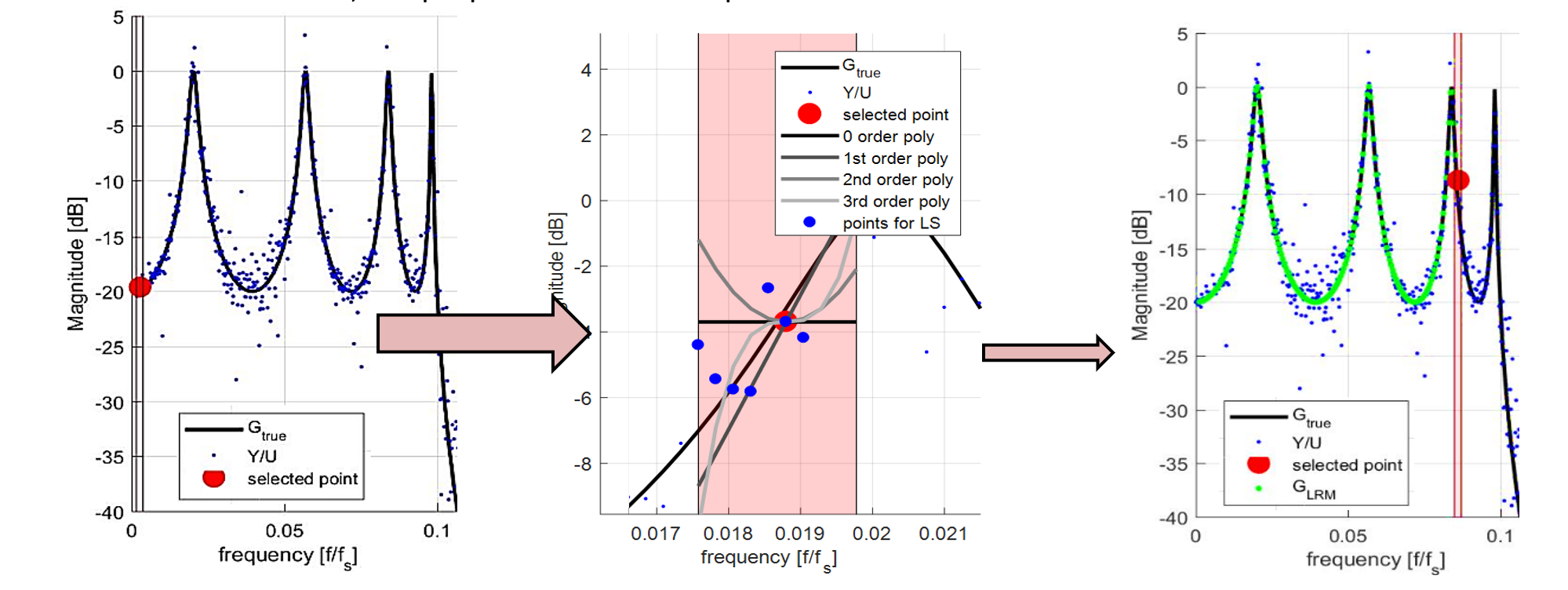
The suggested local polynomial/rational method. The figure on the left shows the selection of an excited frequency line and the narrow processing band. The middle figure shows the magnification of a such band, together with a conceptual illustration of polynomials. The small blue dots refer to the unprocessed, transient disturbed points of the FRF estimate. On each of these points the LPM/LRM method is called. The right figure shows the moving the narrow processing band. The green dots refer to the new estimated points.
Multiplying the output model equation with D makes all parameters linear that can be easily solved. When D=1, then we have the LPM formula, when D is a polynomial, when have the LRM formula.A measurement example is given in the next Figure. The system under test is the frame of a small vehicle (Simrod battery-operated car) excited from vertical and horizontal directions by shakers. There are in total 20 periods (2 realizations, 5 periods per realization) measured. The illustration shows what happens if only one period of the signal is available. Observe that in each case, the proposed method outperforms the classical H1 estimator.

FRF estimates of a lowly damped vehicle using 10 blocks of data (2 realizations, 5 periods) and 1 block of (transient distorted) data. The proposed method proposed method (LRM) outperforms in each case the classical (H1) method.
The Usage
Introduction
The LPRM toolbox is a user-friendly Matlab based toolbox that supports command line interface and it is compatible with the multisine signal generation MUMI toolbox.The LPRM toolbox has been tested with many simulations, real-life industrial measurements, and it is optimized for MIMO (multiple input, multiple output) experiments by making automated choices to reduce the user-interactions.
The author recommends to start the exploration with typing ‘help LPRM’ and going over the ‘demo.m’ file that contains a series of demonstrations based on a real-life industrial measurement that is shown in the figure above.
The user can directly use the toolbox without setting any parameters, like in ‘LPRM(input,output)’ format. In the ideal case, metadata are available and it can be used to segment the measurement. Such metadata contain, for instance, the sampling frequency (denoted by ‘fs’ in the toolbox), the period length (denoted by ‘N’), the number of periods (denoted by ‘P’) and the number of realizations (denoted by ‘R’). If no meta information is available, in most of the cases, it is possible to use automated data segmentation that is based on the measurement data only. It is done via a simplified statistical process.
If the estimated SNR of the output is adequate (the threshold level is defined in ‘Test_settings.m’ file), then LRM method is used (i.e., ‘solver’ field is set to ‘LRM’), otherwise LPM method is used (i.e., ‘solver’ field is set to ‘LPM’). Optionally, one can use the classical H1 estimator (by setting the ‘solver’ field to ‘H1’).
Preprocessing the measurements
In case of multiple inputs, the toolbox first checks if the input signals are uncorrelated. A MIMO FRM estimation procedure ideally requires independent (uncorrelated) excitation signals. Using multiple channels, it can easily happen that by mistake two or more input channels share the same signal. The automatic processing warns the user, if the correlation is greater or equal than the predefined threshold level that can be found in the ‘Test_settings.m’ file. An example for this situation can be found in the ‘demo.m’ file.The next pre-processing step includes the determination of the period length and the periodicity that is performed by using advanced correlation-based techniques. Once the length of the period (block) N is estimated, the number of periods P has to be estimated. If there are at least three periods (block) available, then the transient check-up algorithm is called. If there are less than three transient-free periods, then the FRM estimation is calculated with the transient estimation method (i.e., ‘estimateTransient’ options is set to ‘1’), otherwise, the transient disturbed periods (blocks) are discarded and the ‘estimateTransient’ options is set to ‘0’).
If there is mismatch between the results of the automated segmentation and meta data information, then the user is warned (see the ‘demo.m’ file for an illustration).
Estimation process
For computational optimality, the FRM estimation is solved output-channel-wise (i.e., one output channel per unit time). The FRM estimate is calculated at the excited frequency lines only. The toolbox tries to automatically determine the excited frequency lines (that are stored in the ‘ind.exc’ field). This process can be tuned by setting manually the field ‘RMSthreshold‘ (that refers to the excitation threshold in dB scale) or providing the excited lines by overriding ‘ind.exc’ field. The whole frequency scale can be found in the ‘f’ field (these values correspond to Hz values). In the frequency band of excitation (i.e., between the (automatically determined) values ‘fmin’ and ‘fmax’ fields), the FRM estimates at the non-excited bins are obtained by (linear) interpolation.When there are multiple R realizations, a partial FRM estimate is obtained via averaging over the P periods (blocks) in a realization. The partial estimates can be found in the ‘G_m’, ‘U_m’, ‘Y_m’ fields that correspond to the FRM, input and output spectra estimates. After the 2D averaging (i.e., averaging over P and R) the total FRM and input-output and transient spectra estimates are obtained (that are stored in ‘G’, ‘U, ‘Y’, ‘T’ variables).
In addition to these, for each FRM and input-output spectra the noise covariances, and multiple coherences are estimated.
Setting up the solver
For each frequency line there are 3d+2 unknown parameters to be estimated (d+1 in Gp, d+1 in Tp, d in D). This means, for the algorithm to work the frequency in the processing window should be at least 3d+2 wide (i.e. |r|≥3d+2). The bandwidth of the processing window can be modified by setting the ‘bw’ parameters. Higher bandwidth will result in smoother estimates, however, too much smoothness can change the damping values (i.e., the peaks of the FRFs). The restriction on the width of the processing window also means that in the FRM measurement, in the -3dB bandwidth of the lowest damped mode (the sharpest peak in the FRF) should be at least 3d+2 points measured. At the edges of the FRM measurement (around the first and last excited bins) the processing window should be modified to include at least 3d+2 points. In order to make use of the smoothness properties of the transfer and transient functions, the polynomials have to be (at least) quadratic. On the other hand, using higher order polynomials will increase the window length that may result in high bias error for lowly damped systems. Therefore, it is recommended to use second order polynomials as a first step.The basic (automated) setting uses second order polynomials (that is denoted in the structure as ‘degree’) and it determines automatically the (minimum) bandwidth (denoted as ‘bw’). If there are fewer number of points than the bandwidth, the user is warned.
Downloads
The toolbox can be downloaded from Github
See also
References - related articles
1. Csurcsia, P. Z.; Peeters, B.; Schoukens, J. (2020). User-friendly nonlinear framework for industrial measurements with multiple inputs. Mechanical Systems and Signal Processing, Volume 145, November - December 20202. Csurcsia, P. Z.; Peeters, B.; Schoukens, J.; De Troyer, T. (2020). Simplified Analysis for Multiple Input Systems: A Toolbox Study Illustrated on F-16 Measurements. Vibration. 3(2), 70-84
3. Csurcsia, P. Z. (2013). Static Nonlinearity Handling Using Best Linear Approximation: An Introduction. Pollack Periodica, 4(1), 1-12.
4. Csurcsia, P. Z. (2015). Part 1: Nemlinearitások detektálása multiszinuszos gerjesztéssel. Elektronet. 24(5), 36-40. (in Hungarian)
5. Csurcsia, P. Z. (2015). Part 2: Nemlinearitások detektálása multiszinuszos gerjesztéssel. Elektronet. 24(6), 44-47. (in Hungarian)
6. Ramaswamy, K. R.; Csurcsia P. Z.; Van den Hof P.; Schoukens J. A frequency domain approach for local module identification in dynamic networks. Automatica
7. Siddiqui, M. F.; De Troyer, T.; Csurcsia, P. Z.; Decuyper, J.; Schoukens, J.; Runacres, M.; A nonlinear state-space model of the unsteady lift force on a pitching wing. Mechanical Systems and Signal Processing
8. Csurcsia, P.Z.; Decuyper J.; Schoukens J.; De Troyer T. A study on decoupling PNLSS models illustrated on an F16 air fighter. Mechanical Systems and Signal Processing
9. Csurcsia, P. Z.; Peeters, B.; P., De Troyer, T. Simplified nonlinearity assessment of MIMO systems illustrated on ground vibration testing. Mechanical Systems and Signal Processing
10. Csurcsia, P. Z.; Peeters, B. Time-varying Operational Modal Analysis using Multidimensional Regularization.
11. Csurcsia, P.Z.; De Troyer T. (2021). An empirical study on decoupling PNLSS models illustrated on an airplane. 19th IFAC Symposium on System Identification. Italy.
12. Csurcsia, P.Z.; Decuyper J.; Schoukens J.; De Troyer T. (2021). Empirical study on decoupling PNLSS models illustrated on F16. Workshop on Nonlinear System Identification Benchmarks. Eindhoven, The Netherlands
13. Van den Bossche, S.; Csurcsia, P.Z. (2021). Modelling of F-16 Ground Vibration Testing Measurements Using Machine Learning Techniques. International Modal Analysis Conference. Orlando, USA
14. Csurcsia, P.Z.; De Troyer T. (2021). Frequency Response Function Estimation for Systems with Multiple Inputs using Short Measurement: A Benchmark Study. International Modal Analysis Conference. Orlando, USA
15. Csurcsia, P.Z.; Decuyper J.; De Troyer T. (2021). Nonparametric Nonlinear Modelling of an F16 Ground Vibration Testing Measurement. International Modal Analysis Conference. Orlando, USA
16. Csurcsia, P. Z.; Peeters, B.; Schoukens, J. (2020). B-spline based time-varying operational modal analysis illustrated on a wind tunnel testing measurement. International Conference on Noise and Vibration Engineering. Leuven. Belgium
17. Csurcsia, P. Z.; Peeters, B.; Schoukens, J. (2020). The Best Linear Approximation of MIMO systems: simplified nonlinearity assessment using a toolbox. International Conference on Noise and Vibration Engineering. Leuven. Belgium
18. Peeters, B.; Csurcsia, P. Z.; Bianciardi, F (2020). Novel MIMO Frequency Response Function estimation technique suited for short measurements: a benchmark study. International Conference on Noise and Vibration Engineering. Leuven. Belgium
19. De Troyer, T.; Csurcsia, P. Z.; Greenblatt D (2020). Nonlinear system identification of a pitching wing in a surging flow. International Conference on Noise and Vibration Engineering. Leuven. Belgium
20. Elkafafy, M.; Csurcsia, P. Z.; Cornelis, B.; Risaliti, E; Janssens, K (2020). Machine learning and system identification for the estimation of data-driven models: An experimental case study illustrated on a tire-suspension system. International Conference on Noise and Vibration Engineering. Leuven. Belgium
21. Siddiqui, M. F., Csurcsia, P. Z.; De Troyer, T.; Runacres M. C. (2020). Development of a nonlinear data-driven model of the lift on a pitching aerofoil. Torque 2020. Delft, the Netherlands
22. Csurcsia, P. Z.; Di Lorenzo, E.; Musella, U.; Hallez, R.; Debille, J.; Peeters, B. (2019). Structural dynamics assessment on a full-electric aircraft: ground vibration testing and in-flight measurements. International Forum on Aeroelasticity and Structural Dynamics. Georgia, USA
23. Csurcsia, P. Z.; Peeters, B.; Schoukens, J. (2019). The Best Linear Approximation of MIMO Systems: First Results on Simplified Nonlinearity Assessment. International Modal Analysis Conference. Orlando, USA
24. Csurcsia, P. Z.; Peeters, B.; Schoukens, J. (2019). Tracking the modal parameters of time-varying structures by regularized nonparametric estimation and operational modal analysis. 2019 International Operational Modal Analysis Conference. Coppenhagen, Denmark
25. Csurcsia, P. Z.; Schoukens, J.; Peeters, B. (2018). Regularized time-varying operational modal analysis illustrated on a wind tunnel testing measurement. International Conference on Noise and Vibration Engineering. Leuven, Belgium
26. Luczak, M.; Peeters, B.; Manzato, S.; Di Lorenzo, E.; Csurcsia, P. Z.; Reck-Nielsen, K.; Ruffini, V. (2018). Integrated dynamic testing and analysis approach for model validation of an innovative wind turbine blade design. International Conference on Noise and Vibration Engineering. Leuven. Belgium
27. Alvarez Blanco, M.; Csurcsia, P. Z. ; Carrera, A. ; Peeters, B. (2018). Nonlinearity Assessment of MIMO Electroacoustic Systems for Direct Field Environmental Acoustic Testing. 31st Aerospace Testing Seminar. Los Angeles, USA
28. Alvarez Blanco, M.; Csurcsia, P. Z.; Peeters, B.; Janssens, K.; Desmet, W. (2018). Nonlinearity assessment of mimo electroacoustic systems on direct field environmental acoustic testing. International conference on Noise and Vibration Engineering. Leuven, Belgium.
29. Csurcsia, P. Z.; Schoukens, J.; Peeters, B. (2018). Nonparametric Approximation of the Nonlinear SilverBox Data: a Linear Time-varying Approach. Workshop on Nonlinear System Identification Benchmarks. Liege, Belgium
30. Csurcsia, P. Z.; Ramaswamy, K. R.; Van den Hof P.; Schoukens J (2021). A frequency domain approach for local module identification in dynamic networks. Workshop of the European Research Network on System Identification. The Netherlands
31. Csurcsia, P. Z., Peeters, B. (2020). User-friendly Nonparametric Framework for Vibro-acoustic Industrial Measurements with Multiple Inputs. Benelux Meeting on Systems and Control. The Netherlands
32. Peeters, B., Csurcsia, P. Z. (2019). Structural nonlinearities - an industrial view. Workshop on Nonlinear System Identification Benchmarks. Eindhoven. The Netherlands
33. Csurcsia, P. Z., Peeters, B., Schoukens, J. (2019). An industrial nonparametric framework for measurements of nonlinear systems. ERNSI Workshop on System Identification. The Netherlands
34. Peeters, B., Csurcsia, P. Z. (2018). The use of exotic multisines in MIMO structural dynamics and acoustic applications. Workshop on Nonlinear System Identification Benchmarks. Liege, Belgium